The equations of motion and solutions are derived for the simple pendulum and a general pendulum. Dynamical maps are introduced as a way of handling nonlinear oscillators.
❦
1 The simple pendulum
Consider a simple pendulum consisting of a mass \(m\) fixed by a light but rigid rod of length \(l\). Gravity acts on the mass with a force \(F=mg\) directed straight down.
A simple pendulum. The driving force on the pendulum is gravity which can be resolved into a components along and perpendicular to the rod.
If the pendulum is at an angle \(\theta\) to the vertical we can resolve the gravitational force on the mass into components parallel and perpendicular to the rod. The parallel component will be balanced by the tension \(T\) on the rod so that \(T=mg\cos\theta\) (unless the rod breaks!). That leaves the perpendicular component which will be directed opposing the direction of the angle \(\theta\).
Now we can use the angular version of Newton’s second law:
\[\begin{equation}\label{eq:tau}
\tau = I \alpha = I \ddot{\theta},\end{equation}\]
where \(\tau\) is the torque and \(\alpha = \ddot{\theta}\) is the angular acceleration. The force causing the torque and the rod are perpendicular so the torque is easy to write down:
\[\begin{equation}\label{eq:tausimple}
\tau = -l m g \sin\theta.\end{equation}\]
The negative sign is because the torque is opposing the angular displacement \(\theta\)—for instance use the right-hand rules to determine the directions of \(\theta\) and \(\tau\). For the simple pendulum the moment of inertia is that of a mass at a distance \(l\) from the pivot so we have \(I=l^2m\) and Eq \eqref{eq:tausimple} reduces to
This is a nonlinear second order differential equation, however if we restrict our attention to small angles so that \(\sin\theta\approx\theta\), then the equation becomes the familiar equation of motion of a harmonic oscillator (with the substitution of \(\theta\) for \(x\)):
where the angular frequency is \(\omega_0 = \sqrt{g/l}\). For details see harmonic-oscillator.
Note: the angular frequency \(\omega_0\) is not the same as the angular velocity \(\dot{\theta}\) which unfortunately tends to be given the same synbol \(\omega\)!
Given the angular frequency, the period of motion is \(T=2\pi/\omega_0 = 2\pi\sqrt{l/g}\) which is independent of the mass and starting angle. This is one of the reasons pendulums make good clocks.
We made a couple of assumptions in the derivation of the equation of motion, one was to assume that the pendulum was effectively a point mass on the end of a negligible rod or string, the other was to assume small angles only. We’ll generalise the treatment in the next sections.
2 Physical pendulum
With an arbitrary shaped pendulum such as that depicted below, we can keep the initial steps of the analysis above.
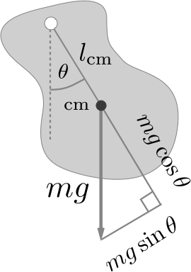
A arbitrarily shaped pendulum. The entire mass of the pendulum acts like it's concentrated at the centre of mass for the torque, but the distribution of mass determines the moment of inertia.
As far as the torque is concerned the force of gravity acts through the objects centre of mass (cm) so \eqref{eq:tausimple} is still valid with the pendulum’s length being the distance between the pivot and the centre of mass \(l_\mathrm{cm}\). Combining equations \eqref{eq:tau} and \eqref{eq:tausimple} rearranging we have
If the angle \(\theta\) is small we can again make the approximation \(\sin\theta\approx\theta\) and arrive at an equation of motion for a harmonic oscillator:
for which the angular frequency is \(\omega_0 = \sqrt{mgl_\mathrm{cm}/I}\). Of course, in practice calculating \(I\) and \(l_\mathrm{cm}\) for some arbitrary shaped object may be quite a challenge.
3 The nonlinear pendulum
In the simple pendulim section we made the simplifying assumption that the oscillations were small enough that \(\sin\theta\approx\theta\). Without this assumption the resulting equation of motion is nonlinear. There is a closed-form solution but it ain’t pretty.
As practice we will rederive the equation of motion using the energy. The kinetic energy will be
So either \(\dot{\theta}=0\) (the pendulum is motionless) or the term in the brackets is zero and we recover the equation of motion we obtained earlier \eqref{eq:eqmotionsimple}:
If \(E\ge mgl\), the rightmost term will be real and will look roughly sinusoidal. For \(E < mgl\) this approach will give complex solutions so let’s take a different tack. For small \(\theta\) we can expand \(\cos\theta\) to second order
This is an equation of an ellipse—quite different behaviour from when \(E\ge mgl\).The behaviour of the pendulum splits into two regions in the \(\theta\)-\(\dot{\theta}\) plane. Above the threshold energy \(mlg\) it looks like a squashed sinusoid, below the threshold and for small \(\theta\) it's an ellipse.
So what is this mysterious transition that happens when \(E=mgl\)? Well, this is just the energy that the pendulum would have if it was started at the very top of its swing! Now its clear what the two behaviours are: will less energy than this critical energy the pendulum swings back and forth as usual, with more energy than the threshold the pendulum keeps doing loops in the same direction.
When we add damping to the pendulum, or look at other nonlinear oscillators then it will often be the case that they will not be amenable to an analytic treatment. The diagram we’ve drawn though will be immensely useful. It forms part of a field called dynamic systems theory and it’s called a dynamical map. A point in the \(\theta\)-\(\dot{\theta}\) space gives the initial conditions for a system, and because we have the change with time of each axis (\(\dot{\theta}\) and \(\ddot{\theta}\)) then we can plot how the system evolves from a given initial condition and so plot flows. By locating and examining particular features in such a space, such as fixed points, we can tell a lot about the behaviour of the system without directly solving the equations of motion. A closely related space is the phase space of a system which is used extensively in the Hamiltonian picture of classical mechanics, instead of the velocities we would plot the momenta.
The simple pendulum's dynamical map. An initial setting of \(\theta\) and \(\dot{\theta}\) is a point in the diagram, the arrows indicate how the pendulum would behave from there. The dashed red line is the boundary between the two types of solution - oscillating back and forth and looping around in a circle.